Originally posted on medium
Cancelations can be a silent killer for e-commerce businesses, eroding revenue and damaging customer relationships. After analyse the success purchase on the The Look E-commerce dataset on this medium article, now we are going to analyse why users canceling their purchase.
This article aims to uncover the underlying factors contributing to order cancellations at The Look E-commerce and provide insights for potential improvements
Note : The data used in this analysis is fictional data and was cerated by Looker team for exploration purpose. While the specific findings may not be directly applicable to real-world scenarios, the methodologies and insights presented can serve as a valuable guide for exploring e-commerce datasets and deriving actionable recommendations.
 1
 2
 3
 4
 5
 6
 7
 8
 9
10
11
12
13
14
15
16
17
18
19
20
21
22
23
|
-- SQL query to get the data for analysis
SELECT
  o.*,
  u.age,
  u.country,
  u.latitude AS user_lat,
  u.longitude AS user_lon,
  u.traffic_source,
  oi.sale_price AS sale_price,
  inv.product_retail_price,
  inv.product_category,
  inv.product_name,
  inv.product_brand,
  inv.product_department,
  dc.latitude AS dc_lat,
  dc.longitude AS dc_lon,
  dc.name AS dc_name
FROM  `bigquery-public-data.thelook_ecommerce.orders` o
LEFT JOIN `bigquery-public-data.thelook_ecommerce.users` u ON o.user_id = u.id
LEFT JOIN `bigquery-public-data.thelook_ecommerce.order_items` oi ON o.order_id = oi.order_id
LEFT JOIN `bigquery-public-data.thelook_ecommerce.inventory_items` inv ON oi.inventory_item_id = inv.id
LEFT JOIN `bigquery-public-data.thelook_ecommerce.distribution_centers` dc ON inv.product_distribution_center_id = dc.id
;
|
After querying data from Biguery, download the data for analysis in R.
1
2
|
dat <- read.csv('~/Desktop/Project/hugo-blog/static/data/thelook_ecommerce_dataset.csv')
head(dat)
|
 1
 2
 3
 4
 5
 6
 7
 8
 9
10
11
12
13
14
15
16
17
18
19
20
21
22
23
24
25
26
27
28
29
30
31
32
33
34
35
|
##   order_id user_id    status gender              created_at returned_at
## 1      202     161 Cancelled      F 2022-02-22 03:58:00 UTC
## 2      241     195 Cancelled      F 2022-08-26 18:54:00 UTC
## 3      267     219 Cancelled      F 2022-07-17 08:09:00 UTC
## 4      285     233 Cancelled      F 2020-08-19 05:21:00 UTC
## 5      424     346 Cancelled      F 2023-12-04 11:51:00 UTC
## 6      601     490 Cancelled      F 2024-06-21 04:30:00 UTC
##   shipped_at delivered_at num_of_item age       country user_lat    user_lon
## 1                                   1  22        France 48.88459    2.509238
## 2                                   1  38 United States 35.97947 -118.887492
## 3                                   1  12         China 23.00895  113.196905
## 4                                   2  67 United States 30.66803  -87.194823
## 5                                   4  43        France 43.31911    5.988499
## 6                                   1  53         China 37.74177  115.729271
##   traffic_source sale_price product_retail_price product_category
## 1        Display     150.00               150.00          Dresses
## 2         Search      13.00                13.00             Plus
## 3         Search      35.00                35.00        Intimates
## 4       Facebook      50.00                50.00   Pants & Capris
## 5        Organic       8.99                 8.99   Sleep & Lounge
## 6         Search      17.00                17.00  Socks & Hosiery
##                                                             product_name
## 1                       Design History Women's Zig Zag Sequin Mini Dress
## 2                                         Ozone Women's Mona Linen Socks
## 3                     Playtex Women's Secrets Perfectly Smooth Underwire
## 4                                Misses Unionbay Boot Cut Corduroy Pants
## 5 Cami Sets Five Color Choices Sizes (S M L) Up2date Fashion Style#CamRG
## 6                              K. Bell Socks Women's 3 Button Leg Warmer
##     product_brand product_department dc_lat   dc_lon        dc_name
## 1  Design History              Women  29.95 -90.0667 New Orleans LA
## 2           Ozone              Women  29.95 -90.0667 New Orleans LA
## 3         Playtex              Women  29.95 -90.0667 New Orleans LA
## 4        UNIONBAY              Women  29.95 -90.0667 New Orleans LA
## 5 Up2date Fashion              Women  29.95 -90.0667 New Orleans LA
## 6         K. Bell              Women  29.95 -90.0667 New Orleans LA
|
Data Exploration
To begin our analysis, we examined the overall cancellation rate within the dataset. This provided a baseline understanding of the problem’s magnitude and its potential impact on the business. By calculating the percentage of cancelled orders and their associated revenue loss, we established a clear picture of the issue at hand.
 1
 2
 3
 4
 5
 6
 7
 8
 9
10
11
12
|
order_trend <- dat %>%
  mutate(
    year_month = floor_date(as_date(created_at), "month")) %>%
      group_by(year_month) %>%
      summarize(total_order = n_distinct(order_id),
                cancel_purchase = n_distinct(order_id[status=='Cancelled']),
                cancelation_rate = round(cancel_purchase / total_order * 100,2),
                amount = sum(sale_price * num_of_item),
                amount_cancel = sum(num_of_item[status=='Cancelled']*sale_price[status=='Cancelled'])
  )

summary(order_trend)
|
 1
 2
 3
 4
 5
 6
 7
 8
 9
10
11
12
13
14
|
##    year_month          total_order     cancel_purchase   cancelation_rate
##  Min.   :2019-01-01   Min.   :  14.0   Min.   :   1.00   Min.   : 7.14
##  1st Qu.:2020-05-24   1st Qu.: 528.2   1st Qu.:  78.25   1st Qu.:14.34
##  Median :2021-10-16   Median :1273.0   Median : 192.00   Median :14.94
##  Mean   :2021-10-16   Mean   :1832.3   Mean   : 275.07   Mean   :14.97
##  3rd Qu.:2023-03-08   3rd Qu.:2555.2   3rd Qu.: 366.00   3rd Qu.:15.51
##  Max.   :2024-08-01   Max.   :8668.0   Max.   :1360.00   Max.   :27.17
##      amount        amount_cancel
##  Min.   :   3296   Min.   :   824.7
##  1st Qu.:  82898   1st Qu.: 12280.2
##  Median : 222120   Median : 32660.7
##  Mean   : 300877   Mean   : 44802.4
##  3rd Qu.: 405396   3rd Qu.: 59198.4
##  Max.   :1420433   Max.   :224732.5
|
The analysis reveals an average monthly cancellation rate of 14.97%, resulting in approximate revenue losses of $44,802. To understand the trend of cancellations over time, we examined order data by month.
 1
 2
 3
 4
 5
 6
 7
 8
 9
10
11
12
13
14
15
16
17
18
19
20
21
22
23
24
25
26
27
28
29
30
31
32
33
34
35
36
37
38
39
40
41
42
43
44
45
46
47
48
49
50
51
52
53
54
55
|
ggplot(order_trend) +
  geom_col(aes(x = year_month, y = `total_order`, stat="identity", fill="# of Order")) +
  geom_line(aes(x = year_month, y = `cancelation_rate` * 100, color="Cancelation Rate",  group = 1),
  ) +
  scale_color_manual(values="black") +
  labs(title = "Purchase and Cancelation Rate Trend", x = "Month", y = "#of Order") +
  scale_y_continuous(sec.axis = sec_axis(~ . / 10000, name = "Cancelation Rate", labels = scales::percent)) +
  annotate(
    'text',
    x = as.Date("2023-03-01"),
    y = 7000,
    label = 'the number of order trend looks \nupward overtime',
    fontface = 'italic',
    size = 2.5
  ) +
  annotate(
    'curve',
    x = as.Date("2023-05-01"),
    y = 6600,
    yend = 5000,
    xend = as.Date("2024-01-01"),
    linewidth = 0.5,
    curvature = 0.5,
    arrow = arrow(length = unit(0.2, 'cm'))
  ) +
   annotate(
    'text',
    x = as.Date("2020-01-01"),
    y = 3300,
    label = 'the trend of cancellation rates \ntends to be constant overtime',
    fontface = 'italic',
    size = 2.5
  ) +
  annotate(
    'curve',
    x = as.Date("2020-10-01"),
    y = 3100,
    yend = 2000,
    xend = as.Date("2021-05-01"),
    linewidth = 0.5,
    curvature = -0.5,
    arrow = arrow(length = unit(0.1, 'cm'))
  ) +
  theme_classic() +
  theme(legend.key=element_blank(),
          legend.title=element_blank(),
          panel.grid.major = element_blank(),
          panel.grid.minor = element_blank(),
          legend.box="horizontal",
          legend.position= c(.5,.95),
          legend.text=element_text(size=9),
          plot.title = element_text(color="black", size=14, face="bold.italic", hjust=0.5),
          axis.title.x = element_text(color="darkgrey", size=9),
          axis.title.y = element_text(color="darkgrey", size=9)
        )
|
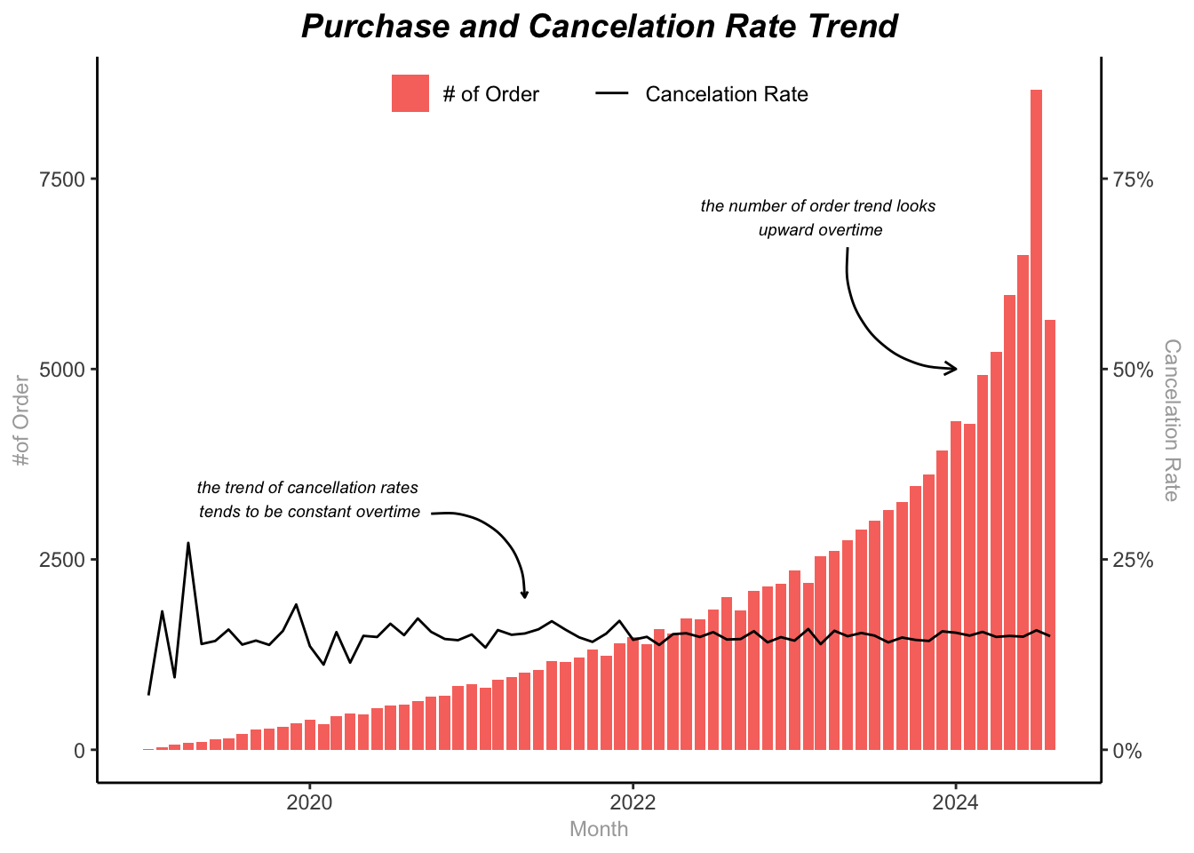
Despite an upward trend in overall order volume, the cancellation rate has remained consistent. This indicates a persistent issue that warrants further investigation. To identify potential causes, we will examine the relations between order status with some variables.
Data Analysis
To enhance our analysis, we conducted feature engineering to create new variables.
- is_cancel : A binary indicator was created, assigning 1 to cancelled orders and 0 to completed orders.
- age_group : Customer ages were grouped into specific intervals to identify potential age-related patterns in cancellations.
- deliver_to : Given the US-based distribution center, a binary variable was created to distinguish between domestic and international orders, exploring potential shipping-related impacts on cancellations.
 1
 2
 3
 4
 5
 6
 7
 8
 9
10
11
12
13
14
15
16
17
18
|
order_dat <- dat %>%
  filter(status!="Processing")%>%
  group_by(order_id) %>%
  summarise(age=mean(age),
            gender=gender[[1]],
            product_department = product_department[[1]],
            traffic_source = traffic_source[[1]],
          total_item = sum(num_of_item),
          total_amount = sum(num_of_item * sale_price),
          is_cancel = ifelse(status == 'Cancelled', 1, 0),
          deliver_to = ifelse(country == "United States", 1, 0) # 0 if deliver to outside US
          ) %>%
  ungroup %>% distinct(order_id, .keep_all = TRUE)
#change categorical data to factor

col <- c("gender","product_department", "traffic_source", "is_cancel", "deliver_to")

order_dat %>% mutate_at(col, as.factor)
|
 1
 2
 3
 4
 5
 6
 7
 8
 9
10
11
12
13
14
15
|
## # A tibble: 99,581 × 9
##    order_id   age gender product_department traffic_source total_item
##       <int> <dbl> <fct>  <fct>              <fct>               <int>
##  1        2    41 M      Men                Search                  1
##  2        3    41 M      Men                Search                  1
##  3        4    41 M      Men                Search                  1
##  4        5    55 F      Women              Search                  1
##  5        6    31 M      Men                Search                  1
##  6        7    68 F      Women              Facebook                1
##  7        8    33 M      Men                Facebook               16
##  8       10    70 M      Men                Display                 1
##  9       12    15 F      Women              Search                  1
## 10       13    15 F      Women              Search                  1
## # ℹ 99,571 more rows
## # ℹ 3 more variables: total_amount <dbl>, is_cancel <fct>, deliver_to <fct>
|
 1
 2
 3
 4
 5
 6
 7
 8
 9
10
|
## # A tibble: 6 × 9
##   order_id   age gender product_department traffic_source total_item
##      <int> <dbl> <chr>  <chr>              <chr>               <int>
## 1        2    41 M      Men                Search                  1
## 2        3    41 M      Men                Search                  1
## 3        4    41 M      Men                Search                  1
## 4        5    55 F      Women              Search                  1
## 5        6    31 M      Men                Search                  1
## 6        7    68 F      Women              Facebook                1
## # ℹ 3 more variables: total_amount <dbl>, is_cancel <dbl>, deliver_to <dbl>
|
Analyse numerical variables vs order status
To understand how numerical variables influence order cancellations, we examined age, total items purchased, and total purchase amount. Before conducting correlation tests, we assessed the normality of these variables using the Kolmogorov-Smirnov test. This test was chosen over Shapiro-Wilk due to its suitability for larger datasets.
H0 : Data follow normal distribution
H1 : Data doesn’t follow distribution
 1
 2
 3
 4
 5
 6
 7
 8
 9
10
11
12
13
14
15
16
|
#normality check

norm_test <- function(variable) {
  ks_test <- ks.test(order_dat[[variable]], y='pnorm') #set y to pnorm since we want test our variables toward normal distribution
  res <- paste0("data :", variable, "  ", "p_value :", ks_test$p.value)
  return(res)
}

#Select only numerical variables
numeric_vars <- c("total_item", "age", "total_amount")

# Calculate the correlation matrix
norm_test_results <- lapply(numeric_vars, norm_test)

names(norm_test_results) <- norm_test_results
norm_test_results
|
1
2
3
4
5
6
7
8
|
## $`data :total_item  p_value :0`
## [1] "data :total_item  p_value :0"
##
## $`data :age  p_value :0`
## [1] "data :age  p_value :0"
##
## $`data :total_amount  p_value :0`
## [1] "data :total_amount  p_value :0"
|
The Kolmogorov-Smirnov test revealed that all three numerical variables (age, total items, and total amount) deviate significantly from a normal distribution (p-value < 0.005). As a result, non-parametric tests are required. To assess differences in these variables between successful and cancelled orders, we employed the Wilcoxon rank-sum test.
H0 : There is no difference (in terms of central tendency) between the two groups in the population.
H1 : There is difference (in terms of central tendency) between the two groups in the population.
 1
 2
 3
 4
 5
 6
 7
 8
 9
10
11
12
13
|
library(ltm)

#function for wilcoxon test
wilcox_test <- function(variable) {
  wilcox <- wilcox.test(order_dat[[variable]][which(order_dat$is_cancel == 1)], order_dat[[variable]][which(order_dat$is_cancel == 0)])
  res <- paste0("data :", variable, "  ", "p_value :", wilcox$p.value)
  return(res)
}

# Calculate the correlation
wilcox_test_results <- lapply(numeric_vars, wilcox_test)

wilcox_test_results
|
1
2
3
4
5
6
7
8
|
## [[1]]
## [1] "data :total_item  p_value :0.434329795381456"
##
## [[2]]
## [1] "data :age  p_value :0.239814229029068"
##
## [[3]]
## [1] "data :total_amount  p_value :0.734469519974685"
|
With p-values greater than 0.05 for all numerical variables, we fail to reject the null hypothesis. This indicates no statistically significant difference in the central tendency (median) of these variables between successful and cancelled orders. Visualizations also confirmed these findings, showing overlapping distributions for both groups.
 1
 2
 3
 4
 5
 6
 7
 8
 9
10
11
12
13
14
15
16
17
18
19
20
|
library(ggpubr)
set.seed(123)

age_bx <- ggplot(order_dat) +
  geom_boxplot(aes(x=as.factor(is_cancel), y=age)) +
  theme_bw()

item_bx <- ggplot(order_dat) +
  geom_boxplot(aes(x=as.factor(is_cancel), y=total_item)) +
  theme_bw()

amount_bx <- ggplot(order_dat) +
  geom_boxplot(aes(x=as.factor(is_cancel), y=total_amount)) +
  theme_bw()

figure <- ggarrange(age_bx, item_bx, amount_bx,
                    common.legend = TRUE, legend="bottom", ncol = 3, nrow = 1)

annotate_figure(figure, top = text_grob("Order Status By Age, Total Item and Total Amount",
               color = "red", face = "bold", size = 12))
|
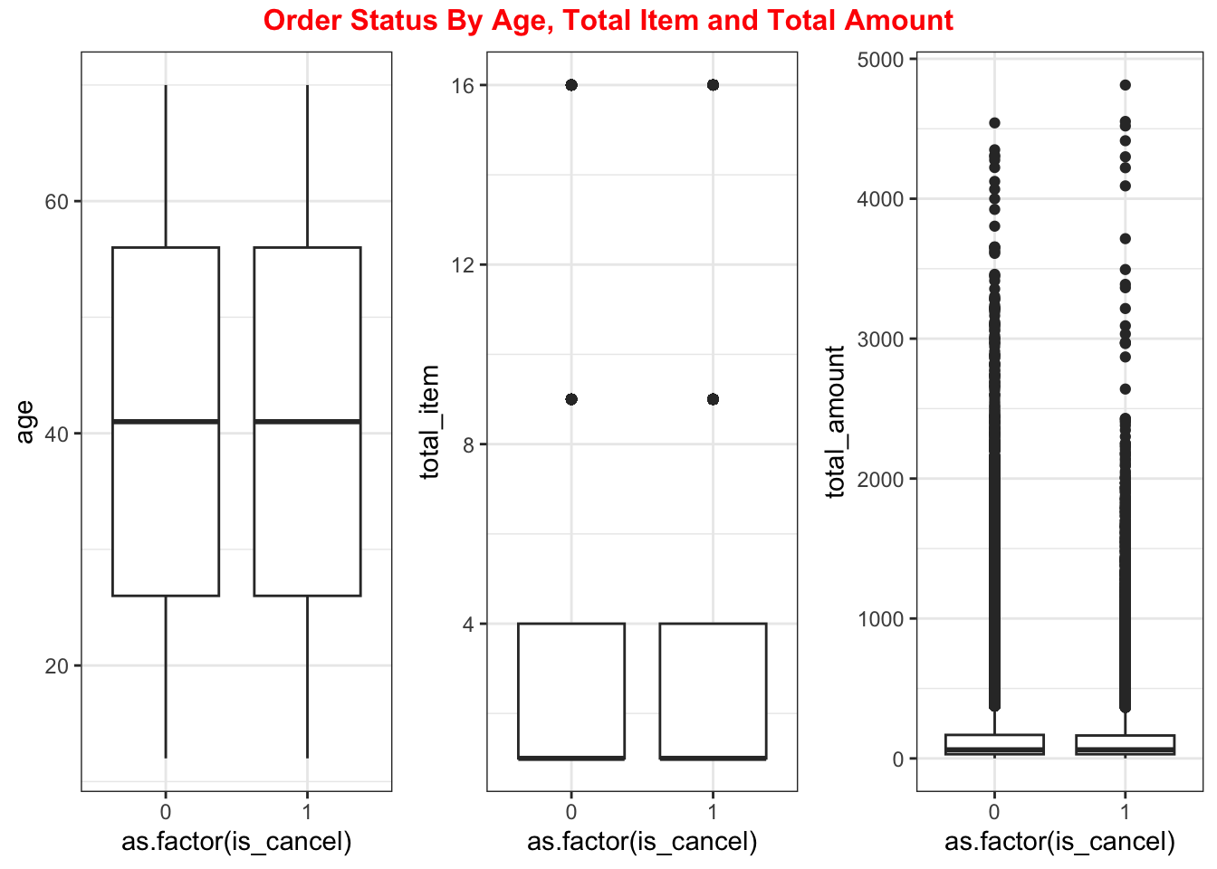
Visualizations also confirmed these findings, showing overlapping distributions for both groups. across age, number of items, or total purchase amount.
- Age of users has no signficant correlation towards order status
- Number of item of purchase has no signficant correlation towards order status
- Total amount of purchase has no signficant correlation towards order status
Consequently, these numerical variables do not appear to significantly influence order cancellation rates.
Analyse categorical variables vs order status
Next, we’ll examine how categorical variables such as product department, age group, traffic source, and delivery destination relate to order cancellations. To determine if there’s a significant association between these variables and order status, we’ll conduct chi-square tests.
H0 : There’s no association between categorical variables and order status
H1 : There’s association between categorical variables and order status
 1
 2
 3
 4
 5
 6
 7
 8
 9
10
11
12
13
14
15
16
17
18
19
20
21
22
23
24
25
26
27
28
29
30
|
# Categorize age group into categorical variables
order_dat <- order_dat %>%
  mutate(
    # Create categories
    age_group = dplyr::case_when(
      age <= 17            ~ "0-17",
      age > 17 & age <= 25 ~ "18-25",
      age > 25 & age <= 34 ~ "26-45",
      age > 45 & age <= 55  ~ "46- 54",
      age > 54  ~ ">55"
    )
)
order_dat$age_group = as.factor(order_dat$age_group)

# Function to perform Chi-Square test for a given variable
chi_square_test <- function(variable) {
  table <- table(order_dat[[variable]], order_dat$is_cancel)
  chisq <- chisq.test(table)
  return(chisq)
}

# List of categorical variables
categorical_vars <- c("product_department", "gender", "traffic_source", "deliver_to", "age_group")

# Apply Chi-Square test to each categorical variable
chi_square_results <- lapply(categorical_vars, chi_square_test)

# Display the results
names(chi_square_results) <- categorical_vars
chi_square_results
|
 1
 2
 3
 4
 5
 6
 7
 8
 9
10
11
12
13
14
15
16
17
18
19
20
21
22
23
24
25
26
27
28
29
30
31
32
33
34
35
36
37
38
|
## $product_department
##
## 	Pearson's Chi-squared test with Yates' continuity correction
##
## data:  table
## X-squared = 1.705, df = 1, p-value = 0.1916
##
##
## $gender
##
## 	Pearson's Chi-squared test with Yates' continuity correction
##
## data:  table
## X-squared = 1.705, df = 1, p-value = 0.1916
##
##
## $traffic_source
##
## 	Pearson's Chi-squared test
##
## data:  table
## X-squared = 4.6306, df = 4, p-value = 0.3273
##
##
## $deliver_to
##
## 	Pearson's Chi-squared test with Yates' continuity correction
##
## data:  table
## X-squared = 0.18457, df = 1, p-value = 0.6675
##
##
## $age_group
##
## 	Pearson's Chi-squared test
##
## data:  table
## X-squared = 3.2614, df = 4, p-value = 0.5151
|
Based on the chi-square test results, here’s a the conclusion:
-
Product Department and Gender: Both tests show identical results (p-value = 0.1916). This suggests no significant association between order status and product department or gender. The similarity in results might indicate these variables are closely related or potentially the same in our dataset.
-
Traffic Source: With p-value = 0.3273, there’s no significant association between traffic source and order status. The different sources (organic, email, social, etc.) don’t appear to influence cancellation rates significantly.
-
Delivery Destination: The test (p-value = 0.6675) indicates no significant relationship between delivery destination (export or domestic) and order status. Whether an order is domestic (US) or international doesn’t seem to affect cancellation rates.
-
Age Group: With p-value = 0.5151, there’s no significant association between age groups and order status. This suggests that cancellation rates don’t vary significantly across different age categories.
In summary, none of the tested variables show a statistically significant association with order status at the conventional 0.05 significance level. This implies that these factors alone may not be strong predictors of order cancellations in our e-commerce dataset.
Findings and Recommendations
The lack of significant correlations suggests that factors beyond the analyzed variables contribute to cancellations. Potential areas for further investigation include:
- Product-related issues: Product quality, descriptions, or images might influence cancellations.
- Customer service: Issues during the checkout process or post-purchase support could impact customer satisfaction.
- Website experience: Website performance, navigation, or mobile optimization might affect the purchase journey.
- Pricing and promotions: Price perception or promotional factors could influence purchase decisions.
- By focusing on these areas, The Look E-commerce can potentially reduce cancellation rates and improve customer satisfaction.
Conclusion
While this analysis identified no direct correlations between the studied variables and order cancellations, it highlights the need for further exploration into other potential factors. Continuous monitoring of cancellation rates and in-depth analysis of specific customer segments are essential for effective retention strategies.
